Virtual Tree¶

First Problem¶

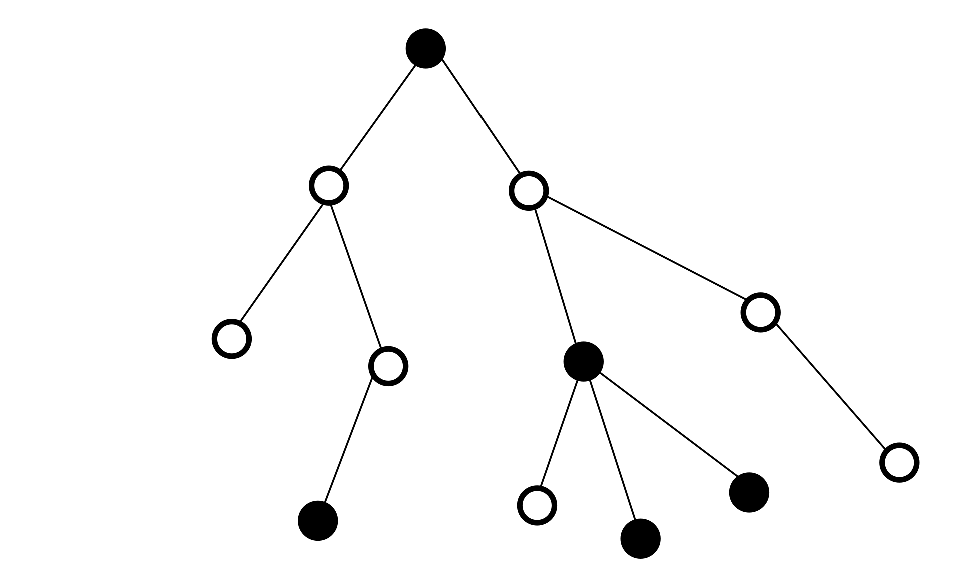
Suppose we have colored a subset of the tree's vertices, say \(B\), black. Now we want to color some uncolored vertices black such that all black vertices become connected. Additionally, we want the total number of black vertices to be minimized. Find this minimum count.

It's clear that to solve this problem, we must color all vertices that lie on the path between at least two black vertices. But the important question is how to find the number of these vertices such that our time complexity depends on \(|B|\) and is completely independent of \(n\). (i.e., if the given set is small, we should answer quickly, and vice-versa).

Let the answer be \(ans\). Note that \(ans\) itself might be very large and not of the order of \(|B|\). For example, if our tree is a path and \(B\) is the set of the two endpoints of this path, then \(ans=n\). Therefore, we cannot work with a time complexity of \(ans\).

Now, pay attention to this interesting point. Consider the final state of the tree (where black vertices are connected) and suppose we define the 'black degree' of each vertex \(u\) as the number of black vertices adjacent to the black vertex \(u\). As you probably noticed from the path example, many vertices we are forced to color black might have a black degree of 2!

We perform an equivalent transformation on the problem to simplify our work. Root the tree at one of the vertices in \(B\). Now, for every vertex \(u\) in \(B\), all vertices from \(u\) up to the root must be colored black, and this coloring is also sufficient (meaning the resulting structure satisfies the connectivity condition).

This is where our problem becomes somewhat similar to the virtual tree problem. Suppose we added enough vertices to set \(B\) such that it became closed under \(lca\). That is, as long as there were two vertices \(u, v\) in \(B\) such that \(lca(u, v)\) was not in \(B\), we had to color \(lca(u, v)\) black and add it to \(B\).

Now, for every non-root vertex \(u\), call its lowest black ancestor its virtual parent, denoted by \(p_u\). Note that the vertices between \(u\) and \(p_u\) are precisely those we mentioned would have a black degree of 2, and there might be many of them. Now, if we count these vertices for all \(u, p_u\) (their count is \(h_u - h_{p_u} - 1\)) and add this value to the current number of black vertices, we will get the answer to the problem.

In this section, we didn't mention a few key points, including:

• How can we find vertices that, if added to set \(B\), will form a virtual tree?

• Why is the maximum number of vertices in the virtual tree related only to \(B\) and not to \(n\)?

We will answer these questions next. It is also worth noting that the problem we posed in this section is just as easily solvable without re-rooting the tree. The re-rooting we performed was solely for ease of explanation!

Diameter of a Subset¶

Suppose you are given a tree \(T\) and a set \(B\). Now you need to name two vertices within \(B\) whose distance from each other is maximal.

We discussed the DFS-based algorithm for finding the diameter of a tree in Chapter 2. Here too, if the vertices of \(B\) are connected, we can use the same DFS algorithm. What if they are not connected? Our current concern is similar to the previous problem. That is, for any two vertices \(u,v\) from \(B\), we want to add all vertices present on the path \(uv\) to \(B\) and then run the DFS algorithm on the resulting graph.

However, in reality, this is not a good method because, as we stated in the previous problem, the number of vertices we might need to add to \(B\) could be very large.

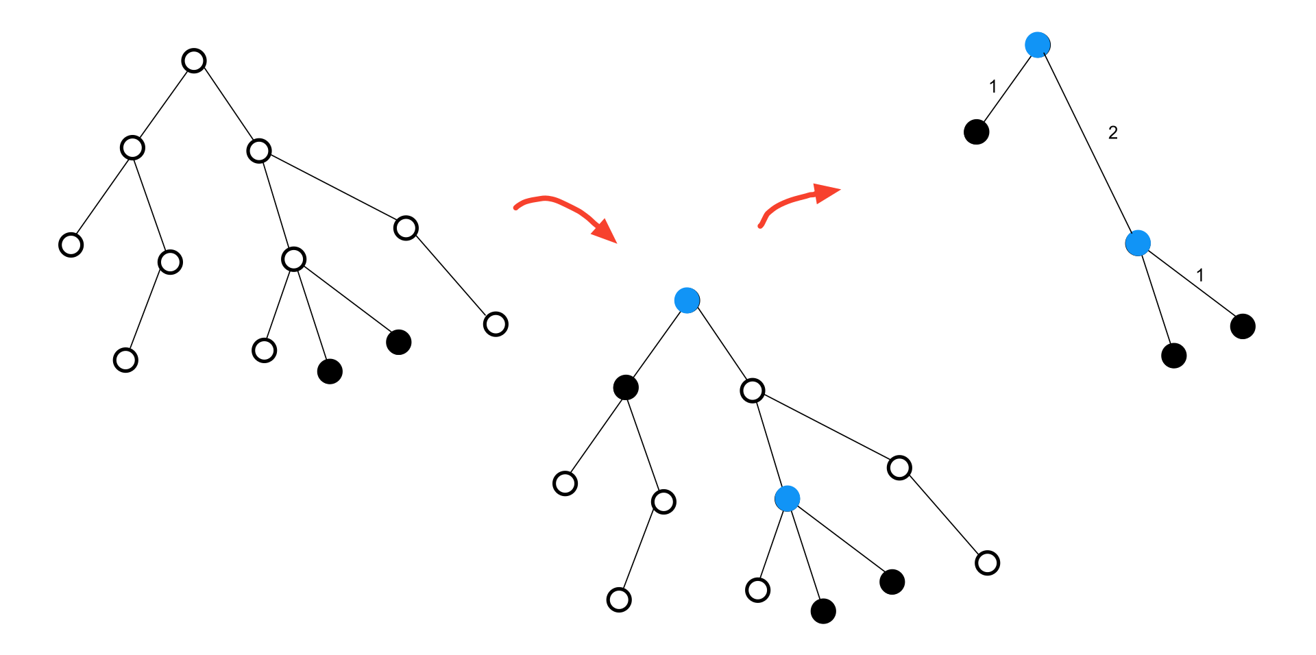
Here, just like in the previous problem, we use the virtual tree. That is, we expand the set \(B\) until it becomes a virtual tree. Now, in a new graph, we draw an edge between each vertex and its virtual parent with a weight of \(h_u - h_{p_u}\). The new tree we have is our virtual tree! By finding the diameter in this tree, we find the maximum distance between the original vertices of \(B\).

Introduction¶

As you probably intuited from the previous problems, a virtual tree can represent a small subtree of our original tree. The interesting point is that this subtree is not necessarily connected, but if we construct a new tree where each vertex is connected to its virtual parent, we obtain a new tree. Then, from now on, we can only consider this new tree and perform our calculations on it.

In this section, we assume that the set of vertices \(B\) is given to us, and we want to add some vertices to it to make \(B\) a virtual tree. Here, we call this process 'expansion'.

First Attempt¶

In the first step, for any two vertices \(a, b\) within set \(B\), we can calculate \(lca(a, b)\) and call this set \(C\).

Now we claim that \(D = B \cup C\) is a virtual tree. For proof, note that every vertex in \(D\) has at least one member of \(B\) within its subtree. (Why?) Now suppose there are two vertices \(a, b \in D\) such that their \(lca\) is not in \(D\). Let \(a\prime\) be a vertex from \(B\) in the subtree of \(a\), and \(b\prime\) be a vertex from \(B\) in the subtree of \(b\). If \(lca(a, b)\) is not in \(D\), then \(lca(a\prime, b\prime)\) would be the same as \(lca(a, b)\), which is in \(C\), contradicting our initial statement.

Therefore, it is sufficient to perform these calculations only for every pair of vertices within \(B\) (and there's no need to check the \(lca\) of newly added vertices with the others).

A Better Algorithm¶

The method we described earlier had high time complexity. If we consider \(lca\) calculations to be \(O(lg(n))\), then the above method would be \(O(|B|^2)\).

Now we try to find a better method. Consider a vertex \(u\) that is not in \(B\) but must be in the virtual tree. This means \(u\) has two children, say \(a\) and \(b\), such that within the subtree of each of \(a\) and \(b\), there exist one or more vertices from \(B\) (whose \(lca\) will be \(u\)).

Now note that taking the \(lca\) of any vertex in \(a\)'s subtree with any vertex in \(b\)'s subtree will yield vertex \(u\). The problem with the previous algorithm was that in these situations, it would calculate \(u\) many times, which we didn't need. That is, for every ordered pair of vertices from \(a\)'s and \(b\)'s subtrees, it calculated vertex \(u\) once, and this is precisely what increased the time complexity of the previous approach.

The interesting point is that if we can define an initial order for the vertices of tree \(T\) such that in this order, each vertex's subtree transforms into an interval, then we can use the following method and claim it works correctly.

• Sort the vertices of \(B\) according to the described order.

• Now, for every two consecutive vertices in the sorted list we obtained, add their \(lca\) to set \(C\).

• The union of the two sets \(B\) and \(C\) forms our virtual tree.

Why does this algorithm work correctly? We said vertex \(u\) has two children, and there's a vertex from \(B\) in each of their subtrees. In the sorted list on which we performed the algorithm, there exists an interval corresponding to the subtree of \(u\). Within the vertices corresponding to this interval, there must definitely be two vertices belonging to the subtrees of different children of \(u\) (Why?) Therefore, when we calculate \(lca\), vertex \(u\) is added to set \(C\)! Just as we wanted.

Optimal Order?¶

In the above algorithm, we magically used an order that had an interesting property. But we didn't provide such an order.

You can construct such an order yourself. All methods for constructing such an order are rooted in the DFS algorithm. Why? Because when we want to calculate this order for the subtree of a vertex like \(u\), we must first recursively find such an order for the subtrees of all of \(u\)'s children, and then add vertex \(u\) somewhere between the intervals of two of its children (or before and after all of them).

This is exactly what we call 'starting-time' or 'finishing-time' in DFS, and we discussed it in Chapter 2.

Implementation¶

const int maxn = 1e5 + 10, max_log = 20;

int start_time[maxn], sparse_table[maxn][max_log], h[maxn];
vector<int> g[maxn];
int Counter = 0;

void dfs(int v, int par = 0){
  h[v] = h[par] + 1;
  sparse_table[v][0] = par;
  for(int i = 1; i < max_log; i++){
      sparse_table[v][i] = sparse_table[sparse_table[v][i-1]][i-1];
  }
  start_time[v] = Counter;
  Counter = Counter + 1;
  for(int u : g[v]){
      if(par != u){
          dfs(u, v);
      }
  }
}

int lca(int a, int b){
  if(h[a] < h[b])
      swap(a, b);
  for(int i = max_log-1; i >= 0; i--){
      if(h[sparse_table[a][i]] >= h[b])
          a = sparse_table[a][i];
  }
  if(a == b)
      return a;
  for(int i = max_log-1; i >= 0; i--){
      if(sparse_table[a][i] != sparse_table[b][i])
          a = sparse_table[a][i], b = sparse_table[b][i];
  }
  return sparse_table[a][0];
}

vector<int> build_virtual_tree(vector<int> vec){
  sort(vec.begin(), vec.end(), [](int a, int b){ return start_time[a] < start_time[b]; }); // sort on starting time
  for(int i = vec.size()-1; i > 0; i--){
      vec.push_back(lca(vec[i], vec[i-1]));
  }
  sort(vec.begin(), vec.end(), [](int a, int b){ return start_time[a] < start_time[b]; });
  vec.resize(unique(vec.begin(), vec.end())-vec.begin());
  return vec;
}

Also, note that if vertex \(u\) is in the virtual tree, and the vertex preceding it in the starting-time order is \(v\), then the virtual parent of \(u\) is equal to \(lca(u, v)\). (Why?)

To calculate \(lca\) in the code above, a method with \(O(lg(n))\) time complexity was used, and finally, finding the virtual tree expansion of set \(B\) was done in \(O(|B| \times lg(n))\) time.