Max-Flow Min-Cut¶

Equality with Min-Cut¶

Consider the same graph from the problem above. We want to remove a set of edges such that there is no directed path from the source vertex to the sink vertex. The goal is to minimize the sum of the capacities of the removed edges. This problem is called the min-cut problem. Below, we will prove that in any graph, the maximum flow is equal to the minimum cut.

Proof¶

First, it is clear that the size of any cut is greater than or equal to the size of any flow. This is because removing any edge reduces the flow by at most its capacity, and as long as there is flow, we have not reached a cut. To prove that the maximum flow is equal to the minimum cut, we consider a maximum flow and construct a cut of the same size.

Consider a maximum flow. An augmenting path is a path with the condition that if we use an edge in its forward direction along the path, its full capacity must not have been used, and if we use it in the reverse direction, there must have been flow passing through it. For example, the following path is an augmenting path:

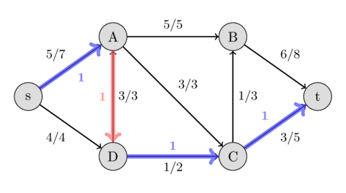
In a maximum flow, there is no augmenting path from source to sink. This is because if one existed, the flow could be increased. It would suffice to increase the flow of edges in the forward direction of the path (the blue edges) by one unit, and decrease the flow of the other edges by one unit. This would increase the total flow by one unit.

Now, to find a cut of size equal to the maximum flow = f, you can consider the vertices that are reachable from the source vertex via an augmenting path. According to the above, the sink vertex is not in this set. The incoming flow to this set is 0, because if there were an edge from outside this set that carried flow into this set, then the vertex outside the set for this edge would also have to be inside this set, as an augmenting path would exist to it. The sum of incoming and outgoing flow for any set of vertices equals the sum of incoming and outgoing flow for each vertex within that set. And the sum of incoming and outgoing flow for each vertex is exactly 0, except for the source and sink vertices. The source vertex has an outgoing flow of f units, so the sum of incoming and outgoing flow for the set we considered is exactly f. Since the incoming flow to this set is 0, the outgoing flow from this set is f. Consider the outgoing edges from this set; all their capacities are fully utilized (otherwise an augmenting path to the vertices external to these edges would exist), and the sum of their capacities is exactly f. If you cut these edges, there is no longer a path from the source to outside this set, and thus no path to the sink. Therefore, we found a cut of size f, which is the size of the maximum flow. Thus, maximum flow equals minimum cut.

Ford-Fulkerson Algorithm for Max-Flow¶

We try to find an augmenting path from the source to the sink and use it to add one unit to the current flow. We continue this process until no more augmenting paths exist. The resulting flow is such that a cut of its size exists. And since we know that all cuts are greater than or equal to all flows, the flow we found is definitely the maximum flow.

The following code snippet implements this algorithm. For simplicity, instead of checking for forward and backward directions separately to find a path, for each edge, we add a reverse edge with a weight of 0. Whenever we pass flow through an edge, we reduce its own capacity and add to the capacity of its dual (reverse) edge.

int cnt, head[M], pre[M], cap[M], to[M], from[M];
int n,m;

void add(int u, int v, int w){
    // adding the original edge
    from[cnt] = u;
    to[cnt] = v;
    pre[cnt] = head[u];
    cap[cnt] = w;
    head[u] = cnt++;
    // adding the dual edge
    from[cnt] = v;
    to[cnt] = u;
    pre[cnt] = head[v];
    cap[cnt] = 0;
    head[v] = cnt++;
}

int tnod = 0;
bitset <M> mark;

// trying to find an augmenting path
int dfs(int u, int mn){
    mark[u] = 1;
    if(u == tnod)return mn;
    // edges of vertex u are stored in a linked list.
    for (int i = head[u]; i != -1; i = pre[i]){
        // if the target edge has no capacity, we ignore it
        if (cap[i] == 0 || mark[to[i]]) continue;
        // trying to find a flow to the sink
        int s = dfs(to[i], min(mn,cap[i]));
        // if s is not 0, an augmenting path exists,
        // and its bottleneck edge has s units of capacity
        if (s){
            // reduce s units from the edge's capacity
            cap[i] -= s;
            // add s units to the dual edge's capacity
            cap[i^1] += s;
            // announce that an s-unit path has been found
            return s;
        }
    }
    // no path found
    return 0;
}

int maxflow(){
    int flow = 0;
    while(1){
        mark &= 0;
        int s = dfs(0, inf);
        // if no path was found, flow = maxflow
        if (!s) return flow;
        flow += s;
    }
}

In this algorithm, we have used the DFS algorithm to find an augmenting path. This algorithm adds at least one unit to the current flow at each step, and since DFS has linear time complexity, this algorithm has a time complexity of \(O(ef)\), where e is the number of edges and f is the maximum flow value. If we used the BFS algorithm instead of DFS, a bound of \(O(ve^2)\) has also been proven, which we will not go into.

Finding Vertex and Edge Connectivity¶

With the help of the max-flow algorithm, vertex and edge connectivity can be found in polynomial time.

To find the edge connectivity, for each undirected edge, we add two directed edges with weight 1 in opposite directions between the two vertices. Then, we find the maximum flow between any two vertices, which is also equal to the minimum cut. Given that the minimum cut does not cut both directions of an edge, the minimum cut of this graph is equal to that of the undirected graph. And every cut disconnects two vertices, so it is greater than the edge connectivity of the graph. Since the minimum number of edges required to disconnect a graph separates two vertices, the minimum of these cuts is the edge connectivity of the graph. The time complexity of this algorithm is \(O(v^3e)\) because the answer is less than the number of vertices.

To find the vertex connectivity of the graph, we construct a new graph where each vertex in the original graph corresponds to two vertices in the new graph: an "in" vertex and an "out" vertex. For each edge in the original graph, we add two edges in the new graph: from the "out" vertex of one endpoint to the "in" vertex of the other, and vice versa. For each original vertex, we also add an edge from its "in" vertex to its "out" vertex. The edges corresponding to the original edges have infinite capacity, and the edges within each vertex (from "in" to "out") have a capacity of 1. To determine how many vertices need to be removed to disconnect two given vertices, we can find the minimum cut between these two "in" vertices (or "out" vertices) in the new graph. We compute this value for all pairs of vertices to find the vertex connectivity. The time complexity of this algorithm is \(O(v^3e)\) because the answer is less than the number of vertices.